SCOPE 13 - The Global Carbon Cycle
12
|
Carbon in the Freshwater Cycle
|
|
S. KEMPE |
ABSTRACT
Annually 1.08 x 10²⁰ g of water precipitates on to the continents, of which 0.376 x 10²⁰
g runs off in rivers. This water is the motor of erosion and terrigenous biological activity alike. The amount of CO2 in rain is small (0.065 x
1015 g C/year) compared with the amount which enters the-water in the soil (net flux reaching the oceans: 0.23 x 10¹⁵ g C/year). Some 0.8 % of all CO2 produced by root respiration and microbial activity reaches the ocean by water transport. The gross flux from soil to groundwater, however, is larger, because much of the CO2 is given off when groundwater reappears in springs. CO2 pressures are 100 times larger in soil air, and 10 times larger in shallow groundwater and in rivers, than in the atmosphere. Both ground and river waters show pronounced seasonal variability of CO2 pressure and alkalinity. An estimated 20% of carbonate rocks occurs in the crust, but only 4% of the continental area shows karst features. These areas play
a distinct role in the carbonate dissolution rate; Europe, the continent with the highest karst percentage, has the largest carbonate concentrations in its rivers.
12.1 INTRODUCTION
The continental fresh waters contain the most diversified carbon pool on earth. Not only does fresh water act as a storage for various inorganic and organic compounds, but it is also a chief transport medium between some of the sizewise more important carbon storages in the biota, lithosphere, and oceans. Furthermore, water is a necessary reaction partner of carbon dioxide, both in the carbonate system and in the biological formation of organic matter. To carry out photosynthesis, land biota is totally dependent on the availability of water (see
Chapter 8, this volume, Figure
8.2).
This chapter provides an introduction to the global water cycle, and a discussion of the different water compartments and their respective carbon contents.
12.2 THE WATER CYCLE
Fresh water is available as precipitation (rain, snow, or dew), ice, rivers, lakes, and ground water. The best values of the global water cycle currently available have
been calculated by Baumgartner and Reichel (1975). Figure 12.1 illustrates the global water cycle: annually 4.25 x 10²⁰ g of water evaporates from the oceans; this is equivalent to a water layer, 117.8 cm thick, spread over the total ocean surface. A total of 0.397 x
1020 g is transferred from the oceans to the continents (11 cm). The continents receive a precipitation of 1.081 x 10²⁰ g annually, equivalent to a layer of 74.6 cm covering the total land area. Of this amount, two-thirds re-evaporate and one-third returns in rivers and glaciers to the sea. The global ratio between evaporation and runoff is 0.357.
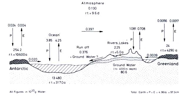
Figure 12.1 The global water cycle (drawn after data by Baumgartner and Reichel, 1975). P = precipitation, E = evaporation, r.t. = residence time
Table 12.1a lists some estimates of the sizes of various water reservoirs. It must be noted that there is no accepted value for the total volume of rivers and lakes available; estimates deviate by as much as a factor of 10. But it is this relatively tiny fraction of water which man most urgently needs, and which he most criminally misuses. Even less information is available for groundwater volumes. Estimates depend on assumptions of mean porosity, mean sediment depth, and mean depth of groundwater table.
Table 12.1b compiles the data for continental runoff and its carbon load. The most recent attempt to make a global calculation of the amount of river loads was made by Livingstone (1963). In
Section 12.10 some corrections are made to the Livingstone calculations: these corrections include updated values for river discharge. Corrections on mean dissolved matter concentrations of the major rivers also seem to be necessary. For many rivers, long-term weighted means are available today, while Livingstone used only data from random sampling.
As rivers provide the bulk transportation from land to ocean
(Table 12.2), their average loads are of primary interest for the carbon cycle. The second largest
discharge rate of eroded material is due to glaciers, while minor amounts are transported by ground water, atmospheric dust, volcanic events, and shore erosion.
Table 12.1a Water volumes of the earth in solid, liquid, and gaseous forms. (Table 1, Baumgartner and Reichel, 1975. Reproduced by permission of the R. Oldenbourg-Verlag GmbH, München)
|
|
|
|
|
|
|
|
|
|
|
|
1015 g |
|
% |
|
|
|
|
|
|
|
1 348000 000 |
|
|
|
Polar ice caps, icebergs, glaciers | |
|
|
|
|
|
Groundwater, soil moisture | |
|
|
|
|
|
|
|
|
|
|
|
|
|
|
|
|
|
|
|
1 384 120 000 |
|
|
|
|
|
|
|
|
|
Fresh water as a percentage of total | |
|
|
|
|
|
Polar ice caps, icebergs, glaciers | |
|
|
|
|
| Ground water to 800 m depth |
|
|
|
|
|
Ground water from 800 to 4000 m depth | |
|
|
|
|
|
|
|
|
|
|
|
|
|
|
|
|
|
|
|
|
|
0.003
|
|
|
|
|
|
|
|
|
|
|
|
|
|
|
|
|
|
|
|
| Various estimates of masses of the hydrosphere (Units in 1015 g H2O) |
| |
|
|
|
|
|
Lvovich |
Flohn |
Garrels et al. |
% |
|
(1970) |
|
(1973) |
|
(1975) |
|
|
|
| Oceans |
1 370 000 000 |
|
1 370 000 000 |
|
1 370 000 000 |
|
80 |
| Pore water in |
60 000 000 |
|
|
|
320 000 000 |
|
18.8 |
|
rocks |
|
|
|
|
|
|
|
| Soil water |
|
|
21 000 |
|
|
|
|
| Groundwater |
|
|
4 00 0000 |
|
|
|
|
|
(750 m) |
|
|
|
|
|
|
|
| Ice |
24 400 000 |
|
27 000 000 |
|
16 500 000 |
|
1.2 |
| Lakes and rivers |
231 000 |
|
116 000 |
|
34 000 |
|
0.002 |
| Atmosphere |
12 400 |
|
|
|
10 500 |
|
0.0006 |
|
12.3 CARBON IN PRECIPITATION
The freshwater cycle starts with 1020 g of water falling annually as precipation on the continents
(Fig. 12.1). The precipitation should chemically assume equilibrium with the atmosphere.
Table 12.1b Annual river discharge and carbon content
|
|
|
|
|
|
|
|
|
|
|
|
|
|
|
| Salinity |
HCO3 | |
|
|
|
|
|
|
|
ppm |
1015 g H2 O |
|
|
|
|
|
|
|
|
|
|
|
|
|
|
|
|
|
|
|
|
|
|
|
|
|
|
|
|
|
|
|
|
|
|
|
|
|
|
|
|
|
|
|
|
|
|
|
|
|
|
|
|
|
|
|
|
|
| weighted means |
|
|
|
|
|
|
Dissolved Organic Carbon (DOC): | |
|
|
|
|
| Particulate Organic Carbon
(POC): |
|
|
|
|
|
Discharge of carbon (in 1015 g/year)
as | |
|
|
|
HCO3 | |
|
|
|
|
|
|
|
|
|
|
|
|
|
|
|
|
Including new data from Amazon River: | |
|
|
|
|
|
With an atmospheric CO2 pressure (PCO2) of 0.0003 parts
CO2 in 1 part of air, we can, according to Henry's law, expect the CO2 content of rainwater to be between I ppm at 0
°C and 0.5 ppm at 20 °C. Because continents and precipitation are unevenly distributed over the climatic zones of the globe
(Figure 12.2 a, b), it is difficult to assess a global mean precipitation temperature. At 15
°C (0.6 ppm CO2), the annual flux with precipitation to the continent surface should amount to
0.6 x 10⁻⁶ CO2 x 1.08 x 1020 g H2 O = 0.065 x 10¹⁵ g
CO2 (0.018 x 10¹⁵ g C/year or 0.0014 x 10¹⁵ moles
CO2 )
Part of the CO2 is instantaneously lost again into the atmosphere, when the precipitation evaporates from rocks, soil, or vegetation. In this context, the ratio between physical evaporation and biological evapotranspiration should be of interest.
In the more densely populated humic zones of the earth, industrial fossil-fuel burning increases the
CO2 content of air locally and rain may contain larger CO2 concentrations as compared with the global average.
Actual measurements of CO2 in rainwater (Table
12.3) show, in fact, a much larger content than expected from the equilibrium argument. The real flux of
CO2
from atmosphere to land with precipitation may, therefore, be several times larger than previously anticipated. No global data are available on rain concentrations of organic carbon.
Table 12.2 Agents of material transport to oceans (After Garrels
et al., 1975, Table 10. Reproduced by permission from Chemical Cycles and the Global Environment, by Garrels, Mackenzie and Hunt. Copyright ©
1975 by William Kaufman, Inc., Los Altos, California. All rights reserved)
|
|
% of total |
|
| Agent |
transport |
Remarks |
|
| Streams |
89 |
|
Present dissolved load 17%, suspended 72%; |
|
|
|
during geologic past more nearly equal. |
| |
|
|
|
| Groundwater |
2 |
|
Estimate poor, dissolved materials like those |
|
|
|
of streams. Major area of ignorance with |
|
|
|
respect to possible contamination. |
| |
|
|
|
| Dust |
0 |
.2 |
Dust to ocean related to deserts and wind |
|
|
|
patterns. Sahara major source for tropical |
|
|
|
Atlantic. Composition similar to average |
|
|
|
sedimentary rock; many dusts have high |
|
|
|
(30%) organic content. |
|
|
|
|
| Shore erosion |
1 |
|
Silts, muds, and sands eroded from shore- |
|
|
|
lines by waves, tides, and currents. Composition |
|
|
|
like suspended load of streams. |
|
|
|
|
| Ice |
7 |
|
Ground-up rock debris as well as material up |
|
|
|
to sizes of boulders. Chiefly from Antarctica |
|
|
|
and Greenland. Distributed in northern and |
|
|
|
southern seas by icebergs. Composition |
|
|
|
similar to average sediments. |
|
|
|
|
| Volcanic |
0 |
.3 (?) |
Lavas and gases transported from earth's |
|
|
|
interior. Amounts and compositions of |
|
|
|
gases poorly known, but include CO2, CH4, |
|
|
|
H2S, SO2, NH3, H2. Dusts from explosive |
|
|
|
volcanoes may be important in climatic |
|
|
|
control. No one knows how much material |
|
|
|
from volcanoes is new to exogenic cycle. |
|
CO2 in rain alone cannot account for the HCO3 found in rivers. According to
|
H2O + CO2 + CaCO3  Ca(HCO3)2
  Ca 2+
+ 2HCO3
Ca 2+
+ 2HCO3 |
at least half of the stream HCO3 must originally be derived from the atmosphere, i.e. 0.23 x
1015 g C (Table 12.1b).
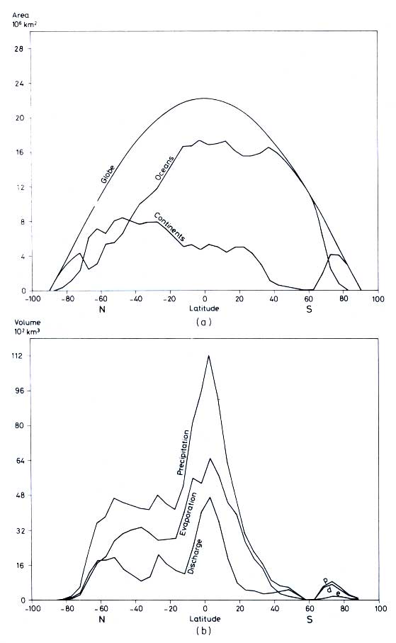
Figure 12.2 (a) Areas of oceans and continents versus latitude
in 5° intervals.
(b) Precipitation, evaporation, and runoff from continents versus latitude in 5 °
intervals (drawn after data by Baumgartner and Reichel, 1975)
Table 12.3 CO2 content of precipitation
(Miotke 1968. Reproduced by permission of the author)
|
|
|
|
|
|
|
|
|
|
|
|
|
|
|
Baumert (1877) in Paul, B. H. | |
|
|
|
|
Peligot (1877) in Paul, B. H. | |
|
|
|
|
|
2.53.5 | |
|
|
|
|
2.22.6 | |
|
|
|
Miotke (1965) Picos, Spain | |
|
|
| |
|
|
|
|
|
|
|
|
|
Bögli (1951) fresh meltwater | |
|
0.851.76 | |
|
|
|
Bögli (1961) from vegetated soil | |
|
2.643.63 | |
|
|
|
Miotke (1965) Picos, fresh meltwater | |
|
|
|
12.4 VOLCANIC CO2
Whether or not volcanic CO2 or CO2 from hydrothermal sources play a quantitatively important role is not yet known. Recycled
CO2, emitted by volcanic vents or moffettes, directly adds to the
atmophere. The estimates of this process differ widely. In certain areas, however, there exists a diffuse
CO2 flow through the crust. These areas are marked by rivers and lakes which carry more bicarbonate than alkaline earth metals. Soda lakes have developed by this process in Ethiopia, Kenya, Tanzania, and in Eastern Turkey (Lake Van;
Kempe, 1977). Crater lakes often have sub-lacustrine CO2 sources, adding volcanic carbon (e.g. Laacher See, Federal Republic of Germany; Lake
Kivu, East Africa).
12.5 SOIL AIR
Additional atmospheric CO2 dissolves in rainwater, only if rain comes into direct contact with alkaline earth metal carbonate rocks. Rain running down bare limestone creates karren by gradual dissolution of CaCO3 and slow uptake of atmospheric
CO2 Bögli, 1975). The final carbonate concentration, however, which these runoff films reach, is far below that of ground or river water.
The major part of CO2 responsible for weathering of carbonates and silicates (see
Chapter 13, this volume) enters precipitation water when it percolates through soil. Due to the immense total surface of soil particles, soil water is in equilibrium with soil air. At this point a substantial amount of
CO2 enters the freshwater cycle.
In soils, bacterial oxidation decomposes the photosynthetically produced organic matter to
CO2. Root respiration is an equally important source of CO2
in soil. CO2 is generated in the. upper few metres of soil, and diffuses upward to the atmosphere and downwards to groundwater. Concentrations and diffusion rates vary with seasons, climate, type of soil, and type of'vegetation cover.
CO2 partial pressures (PCO2) of up to 0.2 have been measured in soils, and an average PCO2 of 0.03 is often quoted
(Miotke, 1974). To monitor CO2 emission from soils, two methods have been followed:
(i) the CO.2 increase in a plastic dome covering the soil surface is measured, and (ii) the apparent diffusion constants of the respective soil profile is determined in the laboratory, together with
CO2 profiles under regular field conditions. Albertsen (1977) has obtained annual averages of
CO2 emissions by this second method for four sites with different vegetation types in Northern Germany: coniferous forest 31 g C/m2 year; deciduous forest 86 g C/m2 year; forest clearing 196 g C/m2 year; and agricultural land 404 g C/m2 year. The bulk
CO2 emission is directed towards the atmosphere; only in spring and early autumn was a concentration gradient towards the groundwater noticed.
The total CO2 content of soil air may be estimated by assuming an average groundwater table depth of 6 m
(Garrels et al., 1975), an average PCO2 of 0.003 (which is certainly on the low side), an average gas effective porosity of 0.2, and a vegetation-covered total continental area of 100 x 106 km2 (see
Chapter 5, this volume, Table
5.2, total continental area minus deserts, semideserts and ice). This calculation yields 36 x 109 m3 of
CO2 of 9.7 x 10¹² g C. As the annual net primary productivity amounts to about 60 x 1015 g C/year
(Chapter 5, this volume), the residence time of
CO2 in soil is approximately one hour. This result is obtained on the assumption that the total primary production is degraded in the soil. This is obviously not the case, as a residence time of one hour is in contradiction with the slow diffusion rate through soil. Therefore, large quantities of litter must degrade under direct contact with the free atmosphere.
The annual net flux of CO2 from soil to groundwater must at least equal the difference between half the
HCO3 load of the streams and the CO2 in rain: 0.23 x 10¹⁵ g C
0.018 x 10¹⁵ g C = 0.21 x 10¹⁵ g C. Garrels et al. (1975) assume that this amount of
CO2 used in the weathering of rocks is derived directly from the atmosphere. As discussed above, this does not seem to be the case. The
CO2 in the process of weathering is derived from 26.5 x 10¹⁵ g C of
CO2 in the model by Garrels et al. (1975) produced by respiration and decay, which then diminishes to about 26.3 x 10¹⁵ g C returning directly to the atmosphere. Consequently the flux of
CO2 used in weathering from the atmosphere to land also diminishes.
The fractionation of degradation CO2 between atmosphere and groundwater is 122/1; 0.77% of the
CO2 produced by degradation of terrestrial organic matter is transferred to groundwater.
With respect to the interaction of water and soil, one other aspect should be noted. If, indeed, most of the
CO2 in groundwater is soil-derived, then this
CO2 must be much older than that furnished by rain. The turnover of humus lapses over a long period, often several hundred years. Reiners (1973) has presented a good review of detritus sizes and turnover masses. Sinter chronology by
14C is limited by the inability to define the time of humus turnover. Double analyses of wood and its sinter cover show the flowstone cover to be much older than the wood, even after
adjusting for the dead CO2 derived from the country rock of the cave roof. It should be possible, by this method, to estimate the fractionation of soil CO2 between percolated water and air.
12.6 TYPES OF RUNOFF
Three types of runoff have to be discerned: overland flow, interflow, and subsurface runoff by groundwater.
Surface runoff is mostly low in dissolved matter, but carries almost all of the suspended particles of the runoff. At times of maximal runoff, the concentration of dissolved substance decreases while suspended load increases.
Interflow occurs through the very upper part of the soil cover, through cracks in the soil, and small surface voids. Interflow behaves hydrologically much like surface runoff, but has geochemical similarities to groundwater.
Groundwater passes totally through the soil and can be clearly discerned geochemically from surface runoff. Its discharge peak after thunderstorms is much delayed or cannot be identified at all. Hydrologists have developed several methods to divide river stage curves into surface and groundwater runoff. These methods, however, are not widely used, and global estimates on the ratio of surface to groundwater discharge have not, as yet, become available.
Three types of groundwater aquifers can be discerned: cleft, porous, and conduit aquifers. The first two have diffuse flow patterns and occur in igneous rocks and shales (cleft), and in sandstones and unconsolidated alluvial rocks (porous). Conduit flow occurs mostly within carbonate karst rocks. Some 80% of the continental surface is covered by sediments, of which 60% are
shales, 20% carbonate rocks, 15% sandstones, and 5% evaporite deposits. The average composition of the sediment cover is slightly different, with 65% shale and 15% carbonates
(Garrels and Mackenzie, 1971; Garrels et al., 1975).
12.7 GROUNDWATER IN KARST ROCKS
The area governed by conduit flow is probably less than 20% of the continental surface, as many calcareous sandstones and shales do not develop conduits. Northern Germany, for example, is underlain by calcareous glacial till, and rivers show high alkalinity and alkaline earth contents similar to karst areas, though hydrologically and morphologically no criteria of karst have been developed.
Balázs (1977a) estimated the total area with morphological karst features to be 4% of the continents
(Table 12.4). The bulk of the karst occurs in Europe and Asia between 60° N and 20° N latitude, with smaller areas in North America and even less in the southern hemisphere
(Figure 12.3). Carbonates occur either in the orogenic belts, or as epicontinental sediments deposited from shallow seas. These areas can form vast karst plateaus once they are uplifted, as in the case of Southern China where the largest single karst area exists. The most pronounced karstification
occurs where limestone and humid climate coincide. Figure 12.4 is a map which shows the main areas of
karst: the AppalachianCaribbean, the European, the South-East Asian and Pacific Karst Provinces
(Balázs, 1977b).
Table 12.4 Distribution of karst areas (Balázs, 1977a. Reproduced by permission of the 7th International Speleological Congress and by permission of the author)
|
|
|
Area of |
Area of karst/1000 km2 |
|
Percentage of karst/ |
|
|
|
continent |
|
|
continent =100% |
|
|
Continent |
106 km2 |
orogenic |
epeirogenic |
Total |
orogenic |
epeirogenic |
Total |
|
|
|
10.5 |
|
|
1418 |
|
|
13.5 |
|
|
|
|
|
1601 |
|
|
|
|
|
|
|
|
|
|
|
|
| North and Central |
24.2 |
|
|
|
|
|
|
|
|
|
|
|
|
|
|
|
|
|
17.9 |
|
|
|
|
|
|
|
|
|
|
|
|
|
|
|
|
|
|
|
|
|
|
|
|
|
|
|
|
|
5341 |
|
|
|
|
|
|
|
|
|
|
|
|
|
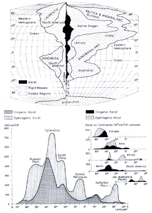
Figure 12.3 Karst areas in comparison to orogen and platform areas in western and eastern hemispheres (top figure). Latitudinal distribution of karst areas in 5° intervals both for total and individual continents
(Balász, 1977a. Reproduced by permission of the 7th International Speleological Congress and by permission of the author.)
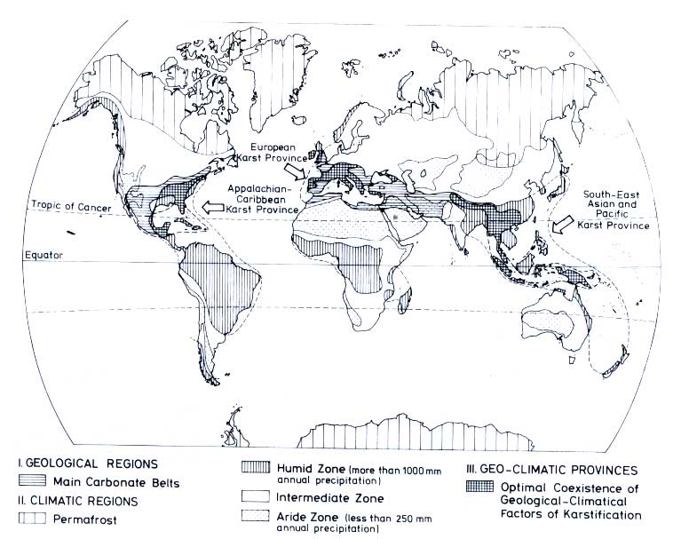
Figure 12.4 Regions of largest geoclimatic potential for karstification
(Balázs, 1977b. Reproduced by permission of the 7th International Speleological Congress and by permission of the author.)
These karst areas play an important role in the bicarbonate budget. Subsurface runoff is the main mode of discharge in
karst. Here, high soil PCO2 (Miotke, 1974) can be neutralized to saturation with calcite (CaCO3) or dolomite (CaMg(CO3)2 ), binding large amounts of CO2. As limestone areas are more common in the humid areas of North America, Europe, and Asia than in the southern continents, we find a very low mean alkalinity in Australian and South American rivers (see
Table 12.1) where hardly any limestone exists. In fact, Europe (with a karst area of 13.5%) has the largest average total dissolved solid
(TDS) concentration (182 ppm) of all the continents. Half of this load is HCO3
(95 ppm).
The complex flow patterns within a carbonate conduit aquifer are illustrated by
Figure 12.5. Very often, air-filled caves intersect the path of seepage water. Most caves exchange their air quite rapidly with the atmosphere. Cave air has, therefore, a lower PCO2 than soil water percolating from above. The water loses
CO2, thus increasing the PCO2 of cave air. Air currents transport the
CO2 back to the surface, where cave mouths are sources of CO2 . When the water loses
CO2, sinter is formed. Where there is no soil above the cave, sinter cannot precipitate, a fact which is best illustrated by
14C flowstone analyses, which show an interruption of sintering in glacial times
(Franke and Geyh, 1972).
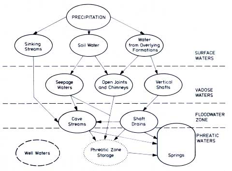
Figure 12.5 Water types encountered in a carbonate
aquifer and their interconnecting flowpatterns (Harmon et al., 1972.
Reproduced by permission of the British Cave Assocation and by permission of the
authors.)
Table 12.5 Karst water analyses (Harmon et al., 1972. Reproduced by permission of the British Cave Research Association and by permission of the authors)
|
|
|
Temp. |
Ca2+ |
Mg2+ |
HCO3- |
pH |
Hardness* |
Hardness† |
SIc |
PCO2 |
Number |
|
|
|
|
|
|
|
|
|
|
log |
of |
|
|
|
|
|
|
|
|
|
|
|
samples |
|
|
GRAND AVERAGES OF KARST WATER TYPES |
|
|
|
|
|
|
|
|
|
|
|
|
|
|
|
|
|
|
|
|
|
|
|
|
|
|
|
|
|
|
|
|
|
|
|
|
5.91 |
|
|
-2.61 |
-0.98 |
|
|
|
|
|
|
|
|
|
|
|
|
|
|
|
|
|
|
|
|
|
|
|
|
|
|
|
|
|
|
|
7.64 |
|
|
+0.11 |
-2.31 |
|
|
|
|
|
|
91 |
7.47 |
|
|
-0.79 |
-2.62 |
|
|
|
|
|
|
|
|
|
|
|
| Zones of fluctuation and phreatic storage |
|
|
|
|
|
|
|
|
|
|
|
|
|
|
|
7.38 |
|
|
-0.60 |
-2.36 |
|
|
|
|
|
|
|
7.77 |
|
|
-0.08 |
-2.60 |
|
|
|
|
|
|
|
7.51 |
|
|
-0.02 |
-2.21 |
|
|
|
|
|
|
|
|
|
|
|
|
|
|
|
|
|
|
|
|
|
|
|
|
|
|
|
|
|
7.30 |
|
|
-0.44 |
-2.14 |
|
|
|
|
|
|
|
|
|
|
|
| REGIONAL AVERAGE OF ALL WATER TYPES |
|
|
|
|
|
|
|
|
|
|
76.2 |
|
|
7.57 |
|
|
+0.08 |
-2.31 |
|
|
|
|
43.5 |
|
|
7.39 |
|
|
-0.45 |
-2.24 |
|
|
|
|
|
|
44 |
7.23 |
|
|
-1.59 |
-2.65 |
|
|
|
|
|
|
|
7.59 |
|
|
-0.14 |
-2.36 |
|
|
|
|
|
|
|
7.56 |
|
|
-0.39 |
-2.52 |
|
|
|
|
|
|
65 |
7.20 |
|
|
-1.50 |
-2.59 |
|
|
|
|
|
|
|
7.78 |
|
|
+0.12 |
-2.61 |
|
|
|
|
|
|
|
6.96 |
|
|
-0.28 |
-1.49 |
|
|
|
|
|
|
|
7.00 |
|
|
+0.17 |
-1.39 |
|
|
|
|
|
|
|
7.13 |
|
|
+0.17 |
-1.57 |
|
|
|
|
|
|
|
|
|
|
|
|
|
REGIONAL AVERAGE OF ALL SPRINGS |
|
|
|
|
|
|
|
|
|
|
|
|
|
7.56 |
|
|
+0.04 |
-2.32 |
|
|
|
|
|
|
|
7.27 |
|
|
-0.61 |
-2.17 |
|
|
|
|
|
|
|
7.44 |
|
|
-0.58 |
-2.46 |
|
|
|
|
|
|
|
7.45 |
|
|
-0.42 |
-2.38 |
|
|
|
|
|
|
|
6.81 |
|
|
-0.35 |
-1.33 |
|
|
|
|
|
|
|
6.84 |
|
|
+0.23 |
-1.14 |
|
|
|
*Hardness as ppm Ca CO3 calculated from Ca2+ + Mg2+ |
|
|
|
|
|
†Hardness as ppm CaCO3 calculated from HCO3-. |
|
|
|
|
With the availability of computer programs for calculating the carbonate equilibria in fresh waters, karst waters have been investigated intensively for their CO2 pressure and mineral saturation. Variation in PCO2, alkalinity, and saturation is due to the length of contact between water and rocks, to the kind of flow encountered, to the mean temperature (and hence to latitude and altitude), and to the seasons.
Table 12.5 compares soil water (top) with water from vadose
and phreatic zones (Harmon et al., 1972). The PCO2 (expressed as a logarithm) of soil water is 0.10, while the saturation index of calcite
(SIc) shows strong undersaturation (negative value). Deeper water still has a PCO2 of 0.05, while the
SIc has reached values near saturation. This water, upon surfacing, loses CO2 until it reaches the atmospheric PCO2 of 0.000 33 (log PCO2
= -3.48) and will precipitate calcite.
The type of flow determines several parameters of the carbonate system. Parizek
et al. (1971), who investigated karst springs with diffuse and conduit flow, found lower total hardness and lower calcite saturation in the case of rapid conduit flow. The variability of hardness is much larger in the conduit compared with the diffuse flow, but CO2 pressure stayed around 0.0032 (log = -2.5) in both groups.
Average composition of karst water is a function of mean temperature
(Figure 12.6, Table 12.5). CO2 pressure and hardness increase at lower latitudes. This is due
to a higher microbial CO2 production in soils of warmer climates, compared to those of cooler regions. For example, PCO2 increases from the northern United States (0.0032, log = -2.5) to Mexico (0.032, log = -1.5) by a factor of 10.
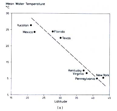
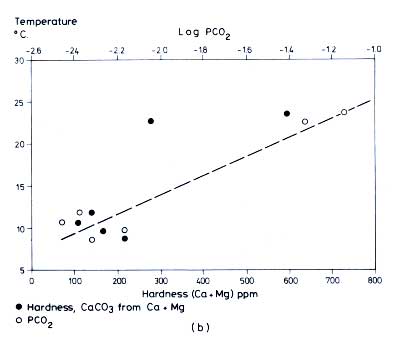
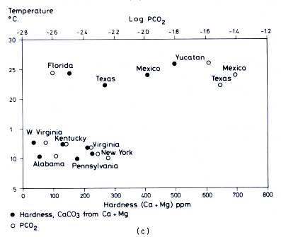
Figure 12.6 (a) Relation between average temperature of karst water samples in
Table 12.5 and latitude (Harmon
et al., 1972). (b) Variation of hardness and PCO2 with water temperature for averages of all samples within a region (compare
Table 12.5) (Harmon
et al., 1972). (c) Variation of hardness and PCO2 with temperature for spring samples only, averaged within the given regions (Harmon
et al., 1972. All figures reproduced by permission of the British Cave Research Association.)
Seasonal variations in PCO2 of karstic waters have been monitored by Hess (1974) in a Pennsylvanian limestone karst and by the Arbeitsgemeinschaft
für niedersächsische Höhlen (unpublished data) in a dolomite and gypsum karst in Germany.
Figure 12.7 gives two log PCO2 curves from the German
karst, depicting a spring from dolomitic source rock with a diffuse flow (annual mean log PCO2
1.7) and a gypsum karst spring with a more or less conduit type of flow (annual mean log PCO2
2.4). The main features of seasonal
CO2 variation in Germany and Pennsylvania show a minimum in CO2 pressure in March-April, due to the beginning of the vegetation period, and a maximum in late summer and autumn, when respiration and decay of organic matter prevail. The amplitude is quite large, over log values of
1.0 in the German and
0.7 in the Pennsylvanian cases. These
figures reveal a pronounced seasonal effect in the CO2 liberation rate from soil. It is, however, not yet possible to calculate from these figures the net flux of inorganic carbon and its seasonal variation. It is known from experience that alkalinity and saturation levels are not only a function of the PCO2, but also of the amount of water present.
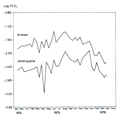
Figure 12.7 Seasonal variation of PCO2 in springs of South Harz mountains, Germany. Top curve: Diffuse flow spring from a dolomite aquifer. Bottom curve: conduit flow spring from a gypsum aquifer (drawn from own data)
12.8 DEEP GROUNDWATER
So far, we have only been concerned with groundwater of the uppermost water-filled zone. Springs discharge water as long as the reservoirs behind them are filled. This gravitational resurging water is dependent on renewal by precipitation in the source area and by the transmissibility of the rock. Low transmissibility will cause slow outflow. The water discharged by springs is mainly recent percolation water, yet a certain amount of older deep groundwater is also involved.
Deep groundwater has very long residence times, up to 1000 or even 10 000 years. The chemistry of deep groundwater (White et al., 1963) is well known in certain areas because of exploration for oil or thermal water. Estimates on the mass of water within the crust differ widely
(Table 12.1).
Many waters (conate waters) have been buried together with the sediments. In tectonically active regions a constant pore-water flux is maintained by compaction. By lowering fresh mud, with 80% porosity, 2 km down into the crust such compaction will occur, and only 10% of the porosity remains
(Wunderlich, 1966). Under such pressures a variety of mineral exchange reactions occur, especially with carbonates. The resurgence of these pore waters is one of the factors which stimulate the circulation of deep groundwater.
12.9 RIVERS
In most cases, groundwater gives off CO2 at its reappearance. If the water stems from
limestones, and is near saturation with respect to calcite, calcium carbonate precipitates downstream. Because of the influence of freshwater biota, most rivers never attain equilibrium of PCO2 with the atmosphere. A characteristic log value for PCO2 in rivers is
2.5. Figures 12.8 and
12.9 depict seasonal variations in PCO2 and alkalinity for the rivers Elbe (23-year mean) and the Amazon (for the year 1975). In the Elbe River,
CO2 pressure and alkalinity decrease with the beginning of the phytoplankton bloom in early spring, with an annual minimum in April. Heterotrophic processes cause the
CO2 pressure to rise quickly to a maximum in July, while alkalinity only slowly regains its former concentrations. A small minimum, caused by a late-summer plankton bloom, is encountered around August and September. The long-term mean of the log PCO2 in the Elbe River is
2.4.
The seasonal PCO2 and alkalinity variation in the Amazon is less regular, though large changes occur during the year. Alkalinity is high during times of spring floods, when more country rocks are exposed to erosion by water. PCO2 is low during
periods of high waters, when nutrients are available to phytoplankton, while larger PCO2 values are encountered during periods of lower waters and the ceasing of photosynthesis.
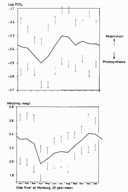
Figure 12.8 Twenty-three-year mean of seasonal variation in PCO2 and alkalinity of the Elbe River at Hamburg (calculated from hydrochemical river records by the Hamburger
Wasserwerke)
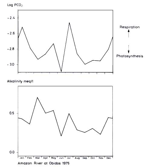
Figure 12.9 Seasonal variation of PCO2 and alkalinity of Amazon River at Obidos 1975 (drawn from data
M.Sc. thesis M. L. Nossar Simöes de Dalgo, personal communication Dra. A. de Luca
Rebello, Rio de Janeiro)
Since the CO2 pressure of rivers is approximately 10 times larger than that of the atmosphere, there must be a considerable flux of
CO2 from stream surfaces into the air. This flux could be estimated according to the laws of diffusion, if we knew the total surface area of streams and their average boundary layer thickness. However, neither figure is available at the moment.
Groundwater also discharges directly into the oceans. This is especially true for limestone areas bordering the sea; half of the drainage of the Yugoslavian
Dinarides, for instance, is said to discharge below sea-level (personal communication, Dr. R.
Gospodaric, Postojna). Water from caves, which developed during glacial times at low sea-level, continues to be transmitted directly to the sea. This water does not come into contact with air again, and, since it stems from carbonate rocks, it carries a substantially greater load of carbon than the global river mean. The size of this flux has not yet been estimated (see
Table 12.2).
With respect to the various parts of the water cycle and the carbon flow interconnected with it, it becomes apparent that the gross flux of carbon from soil to fresh water is probably much larger than that of river loads discharged to the ocean
(Table 12.1 b). How much more carbon that is remains obscure; it may be 50 or even close to 100 per cent of the final discharge.
An attempt is made in Figure 12.10 to show schematically the various fluxes found in the freshwater part of the carbon cycle. Instead of reservoir sizes and flux figures, however, only the PCO2 values and their range in the different compartments are given.
12.10 REVISION OF LIVINGSTONE'S (1963) RIVER LOADS
In 1963 Livingstone published the paper, `Chemical composition of rivers and lakes', which is still the fundamental work for estimating the erosion rates of the continents. By recalculating his world means, several errors, however, became apparent. Both the weighted mean of river salinities of the individual continents and of the world, as well as the HCO3 figure for world runoff are inaccurate.
The weighted mean is calculated by multiplying the volume of discharge with the salinity, adding these figures for continents (or total earth), and dividing this sum by the total discharge for all continents (or total earth):
|
|
 (river discharge x salinity)
 |
|
M (continents)= |
|
|
|
river discharge |
Livingstone obtained a mean world river salinity of 120
ppm. By using his continental means, this figure should read 122.4 ppm. By using recalculated continent values, the salinity is 116.4 ppm and the
HCO3 content becomes 59.8 ppm (instead of 58.4 ppm).
The runoff values quoted by Livingstone have been thoroughly revised by Baumgartner and Reichel (1975)
(Table 12.1b). Using their continent discharge values, in combination with the revised continent salinities of
Livingstone, we obtain a mean total salinity of only 111.06 ppm, i.e. 9 ppm lower (7.5%) than the original value of
Livingstone. This is especially due to the present larger discharges of the Amazon and Orinoco in South America. On the other hand, the total discharged volume has increased
(Livingstone, 32.4 x 10³ km3 /year; Baumgartner andReichel,
37.8 x 10³ km3 /year),which gives a total dissolved load
of 3.77 x 10¹⁵ g/year (revised Livingstone value) and 4.20 x 10¹⁵ g/year (new value) respectively. For HCO3 the Livingstone value is 1.94 x 10¹⁵ g/year (= 0.381 x 10¹⁵ HCO3C g/year) and the new estimate becomes 2.26 x 10¹⁵ g/year (= 0.444 x 10¹⁵ HCO3C/year). There is new chemical data available for some of the larger rivers as well. Livingstone used a mean of 26.4 mg of HCO3 for the Amazon River. Data from the
M.Sc. thesis of Miss Maria Lucia Nossar Simões de Dalgo (courtesy Dra. Angela de Luca
Rebello, Rio de Janeiro, Brazil) indicates an annual weighted mean of 30.4 mg/l. As the Amazon supplies 15.1% of the world runoff, the new mean yields.
|
|
30.4
|
|
|
2.26x10¹⁵ +2.26 x1015 x0.151x |
|
1
= 2.31x10¹⁵ g |
|
|
26.4
|
|
(or 0.454 x 10¹⁵ g HCO3-C/year). This newer value is 19% higher than the revised Livingstone calculations.
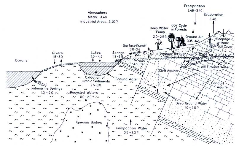
Figure 12.10 -log PCO2 of different freshwater compartments. The CO2 pressure is expressed as its negative decadic logarithm: one unit less means a ten times larger pressure
12.11 POSSIBLE SINKS OF CARBON IN THE FRESHWATER CYCLE
Industry accounts for approximately 5 x 10¹⁵ g of fossil carbon emitted per year into the atmosphere, and possibly the same amount is liberated by land management practices. Of this amount, only 2.4 x 10¹⁵ g stay in the atmosphere while 1.4 x 10¹⁵ g are believed to dissolve in the oceans. The rest enters the carbon cycle at points not yet known. Checking the freshwater cycle for such unnoticed `leaks', we have to keep in mind that the amount of carbon to be looked for surpasses the total flux rates discussed here. We can, therefore, expect only minor sinks in this part of the cycle. Nevertheless, these might exist at several points.
In the most heavily industrialized zones, SO2 emission has decreased the pH of rain below the value of 5.6, which is the normal value, due to the presence of
CO2 and carbonic acid. At a lower pH, the solubility of CO2 increases (one pH unit causes a 100-fold solubility increase; Cole, 1975).
CO2 could, therefore, be lost from the atmosphere faster in polluted areas than in non-polluted regions.
The atmospheric CO2 pressure has risen from a preindustrial value of 0.000 29 to 0.000 33 today (see
Chapter 3, this volume). The rise in
CO2 pressure will certainly increase carbonate dissolution on the continents, though the increase due to carbonate equilibria is only very small. Nevertheless, there is some evidence of an increase in alkalinity and in
CO2 pressure as in the case of the Elbe River (see Chapter
13, this volume), and other rivers can be checked for similarly rising trends. These increases, however, may also be induced by
CO2 released from organic pollution.
In mature woods, CO2 resulting from respiration in soil is quickly recycled by plant uptake, thus keeping the bottom air low in
CO2 . If a forest is cut, this balance is upset in two ways: (i) the total
CO2 production increases (see examples in Section
12.4), and (ii) the
CO2 content of bottom air rises due to lack of large plants to recycle the emitted CO2. Both processes should result in an enlarged
CO2 diffusion to groundwater and hence to an enhanced weathering of rocks.
Also, groundwater usage causes a disturbance in the carbon cycle. Most pumping of groundwater involves the liberation of CO2. On the other hand, younger groundwater, with possibly larger amounts of
CO2, is diverted from the upper levels of the subsurface water body into deeper parts, possibly carrying more
CO2 downwards than the amount of CO2 liberated by the pumping of older ground water.
The eutrophication of fresh water is another process by which we can permanently fix
CO2. Increasing amounts of organic matter are buried in lakes, marshes, and coastal seas.
Probably none of these fluxes will be larger than 1014 g C. Nevertheless, our attempt to investigate them shows how ignorant we are about the flow patterns and flux rates of carbon in connection with the freshwater cycle.
REFERENCES
Albertsen, M. (1977) Labor- and Felduntersuchungen zum Gasaustausch zwischen Grundwasser and
Atmosphäre über natürlichen and verunreinigten Grundwässern. Ph.D. thesis, 1-145,
Christen-Albrechts Universität Kiel.
Balázs, D. (1977a) The geographical distribution of karst areas. Proc. 7th Intern. Congr. Speleology, Sheffield 1977, 13-15, Sheffield.
Balázs, D. (1977b.) The optimal geo-climatic provinces of karstification. Proc. 7th Intern. Congr. Speleology, Sheffield 1977, 15-17, Sheffield.
Baumgartner, A. and Reichel, E. (1975) The World Water Balance, 1-179. R.
Oldenbourg-Verlag, München, Wien.
Bögli, A. (1975) Solution of calcium carbonate and the formation of karren.
Cave Geology 1(1), 1-28 (trans. of the original paper, 1960).
Cole, G. A. (1975) Textbook of Limnology, 1-283. The C. V. Mosby Company, St. Louis.
Flohn, H. (1973) Der Wasserhaushalt der Erde, Schwankungen and Eingriffe. Naturwissenschaften 60(7), 340-348.
Franke, H. W. and Geyh, M. A. (1972). Tropfsteinwachstum and Datierung.
Mitt. Verb. Dt. Höhlen-u. Karstforscher 18(3), 59-60.
Garrels, R. M. and Mackenzie, F. T. (1971) Evolution of Sedimentary Rocks, 1-397. W. W. Norton and Company Inc., New York.
Garrels, R. M., Mackenzie, F. T. and Hunt, C. (1975) Chemical Cycles and the Global Environment, Assessing Human Influences, 3rd ed., 1-206. W.
Kaufmann, Inc., Los Altos, Calif.
Harmon, R. S., Hess, J. W., Jacobson, R. W., Shuster, E. T., Haygood, C., and White, W. B. (1972) Chemistry of carbonate denudation in North America.
Trans. Cave Res. Group of Great Britain 14(2), 96-103.
Hess, J. (1974) Hydrochemical investigations of the Central Kentucky Karst aquifer system. Ph.D. thesis, 1-219, Pennsylania State University.
Kempe, S. (1977) Hydrographie, Warven-Chronologie and organische Geochemie des Van Sees,
Ost-Türkei.
Mitt. Geol.-Paläont. Inst. Univ. Hamburg 47, 123-208.
Livingstone, D. A. (1963) Chemical composition of rivers and lakes. U.S. Geol.
Surv. Prof. Pap. 440G, 1-64.
Lvovich, M. I. (1970) Publ. Assoc. Intern. Hydro. Scient. 93,
401. (Quoted in Flohn, H., 1973.)
Miotke, F. D. (1968) Karstmorphologische Studien in der glazial überformten Höhenstufe
der `Picos de Europa'
Nord-Spanien. Jb. Geogr. Ges. Hannover, Arb. Geograph.
Inst. Techn. Univ. Hannover, Sonderheft 4, 1-161, Selbstverlag
Geograph. Ges. Hannover, Hannover.
Miotke, F. D. (1974) Carbon dioxide and the soil atmosphere. Abh. Karst-
u. Höhlenkunde, R. A 9, 1-49.
Parizek, R. R., White, W. B., and Langmuir, D. (1971) Hydrogeology and
geochemistry of folded and faulted carbonate rocks of the Central Appalachian
type and related land use problems. Min. Conser. Ser., Earth Miner. Sci. Exp.
Station, Circular 82, 1-182, Pennsylvania State University.
Reiners, W. A. (1973) Terrestrial detritus and the carbon cycle. In: Woodwell,
G. M. and Pecan, E. V. (eds), Carbon in the Biosphere. AEC Symp. Ser. 30,
303-327, NTIS U.S. Dept. of Commerce, Springfield, Virginia.
White, D. E., Hem, J. D., and Waring, G. A. (1963) Chemical composition of
subsurface waters. U.S. Geol. Surv. Prof. Pap. 440F, 1-67.
Wunderlich, H. G. (1966) Wesen and Ursachen der Gebirgsbildung, 1-367
Hochschultaschenbücherverlag, Mannheim.
|
Back to Table of Contents |
|
|
|
|
The electronic version of this publication has been
prepared at
the M S Swaminathan Research Foundation, Chennai, India.
|